Tadalafil appartiene alla classe degli inibitori selettivi della fosfodiesterasi di tipo 5, con un profilo farmacocinetico caratterizzato da un’emivita terminale di circa diciotto ore. Dopo somministrazione orale viene assorbito rapidamente e raggiunge concentrazioni plasmatiche massime in due ore. La biotrasformazione avviene principalmente tramite CYP3A4 con formazione di metaboliti inattivi, escreti in prevalenza con le feci. L’elevato legame alle proteine plasmatiche (>90%) assicura una distribuzione stabile. Nei confronti delle altre molecole della stessa classe, cialis compresse italia è noto per la durata prolungata dell’attività farmacologica.
Ed050000561p
Marginal Structural Models to Estimate the Causal Effect of Zidovudine on the Survival of HIV-Positive Angel Herna´n,1 Babette Brumback,2 and James M. Robins1,2
Standard methods for survival analysis, such as the time-
zidovudine on survival and is affected by past zidovudine
dependent Cox model, may produce biased effect estimates
treatment. The crude mortality rate ratio (95% confidence
when there exist time-dependent confounders that are them-
interval) for zidovudine was 3.6 (3.0 – 4.3), which reflects the
selves affected by previous treatment or exposure. Marginal
presence of confounding. After controlling for baseline CD4
structural models are a new class of causal models the param-
count and other baseline covariates using standard methods,
eters of which are estimated through inverse-probability-of-
the mortality rate ratio decreased to 2.3 (1.9 –2.8). Using a
treatment weighting; these models allow for appropriate ad-
marginal structural Cox model to control further for time-
justment for confounding. We describe the marginal structural
dependent confounding due to CD4 count and other time-
Cox proportional hazards model and use it to estimate the
dependent covariates, the mortality rate ratio was 0.7 (95%
causal effect of zidovudine on the survival of human immuno-
conservative confidence interval ϭ 0.6 –1.0). We compare
deficiency virus-positive men participating in the Multicenter
marginal structural models with previously proposed causal
AIDS Cohort Study. In this study, CD4 lymphocyte count is
methods. (Epidemiology 2000;11:561–570)
both a time-dependent confounder of the causal effect of
Keywords: counterfactuals, causality, epidemiologic methods, longitudinal data, survival analysis, structural models, confound- ing, intermediate variables, AIDS.
Marginal structural models (MSMs) can be used to es-
virus (HIV)-positive men enrolled in an observational
timate the causal effect of a time-dependent exposure in
cohort study, the Multicenter AIDS Cohort Study
the presence of time-dependent confounders that are
(MACS). We conclude by comparing methods based on
themselves affected by previous treatment.1,2 The use of
MSMs with previously proposed methods based on g-
MSMs can be an alternative to g-estimation of structural
estimation of SNMs and on the direct estimation of the
In our companion paper we describe inverse-probabil-
We now begin by describing the MACS and then
ity-of-treatment weighted (IPTW) estimation of a mar-
summarize why standard methods for survival analysis
ginal structural logistic model.4 In this paper, we intro-
are not appropriate for estimating the effect of zidovu-
duce the marginal structural Cox proportional hazards
model, show how to estimate its parameters by inverse-probability-of-treatment weighting, provide practical ad-vice on how to use standard statistical software to obtain
The Multicenter AIDS Cohort Study and Bias
the IPTW estimates, and include, as an appendix, the
of Standard Methods
SAS code necessary for the analysis. We use this Cox
Between 1984 and 1991, the MACS enrolled 5,622
proportional hazards MSM to estimate the effect of
homosexual and bisexual men, with no prior acquired
zidovudine on the survival of human immunodeficiency
immunodeficiency syndrome (AIDS)-defining illness,from the metropolitan areas of Los Angeles, Baltimore-Washington, Pittsburgh, and Chicago. Study partici-pants were asked to return every 6 months to complete
From the Departments of 1Epidemiology and 2Biostatistics, Harvard School ofPublic Health, Boston, MA.
a questionnaire, undergo physical examination, and pro-vide blood samples. The design and methods of the
Address correspondence to: Miguel Herna´n, Department of Epidemiology, Har-
MACS have been described in detail elsewhere.5,6
vard School of Public Health, 677 Huntington Avenue, Boston, MA 02115.
We restricted our cohort to HIV-positive men alive in
This research was supported by NIH grant R01-A132475.
the period during which zidovudine was available for use(that is, after study visit 5; March 1986 through March
Submitted March 13, 1999; final version accepted February 28, 2000.
1987). Follow-up ended at study visit 21, October 1994,
Copyright 2000 by Lippincott Williams & Wilkins, Inc.
death, or 24 months after the last visit, whichever came
Epidemiology
first. Our analysis included the 2,178 men who attended
or herpes zoster. We assume, for simplicity, that patients
at least one visit between visits 5 and 21 while HIV
remain on therapy once they start it and that the hazard
positive, and who did not have an AIDS-defining illness
of death at time t depends on a subject’s zidovudine
and were not on antiretroviral therapy at the first eligi-
history only through its current value, but alternative
ble visit. By the end of the follow-up (median dura-
specifications are possible. Suppose, for the moment, no
tion-69 months), 1,296 men had initiated zidovudine
censoring occurs, that is, death times T are observed for
The usual approach to the estimation of the effect of
In the presence of time-dependent covariates L(t)
a time-varying exposure, such as zidovudine, on survival
satisfying the conditions 1 and 2, the estimate ␥ˆ ob-
is to model the hazard of failure at a given time as a
tained by maximizing the Cox partial likelihood is an
function of past exposure history using a time-dependent
(asymptotically) unbiased estimate of the association
Cox proportional hazards model. Robins7 has shown this
parameter ␥ . However, it is a biased estimate of the
approach may be biased, whether or not one further
causal effect of zidovudine on mortality, even if we had
adjusts for past covariate history, whenever (1) there
included the time-dependent covariates L(t) as regres-
exists a time-dependent covariate that is both a risk
factor for mortality and also predicts subsequent expo-
Arguing as in our companion paper,4 we can eliminate
sure and (2) past exposure history predicts the risk fac-
or reduce this bias by fitting the above time-dependent
tor. Covariates satisfying condition 1 are called time-
Cox model with the contribution of a subject i to a
dependent confounders. Past CD4 count is a time-
risk-set calculation performed at time t weighted by the
dependent confounder for the effect of zidovudine on
survival, because it is a risk factor for mortality and a
predictor of subsequent initiation of zidovudine thera-
py,6 and past zidovudine history is an independent pre-
int͑t͒ pr͑ A͑k͒ ϭ a ͑k͉͒A͑k Ϫ 1͒ ϭ a ͑k Ϫ 1͒, V ϭ v ͒
dictor of subsequent CD4 count.8 In fact, all standard
methods (for example, Cox or Poisson regression) that
pr͑ A͑k͒ ϭ a ͑k͉͒A͑k Ϫ 1͒ ϭ
predict the mortality rate at each time using a summary
͑k͒ ϭ li k͒)
of zidovudine history up to that time may produce biasedestimates of the causal effect of zidovudine whether or
to obtain an IPTW partial likelihood estimate. In the
not one adjusts for past CD4 count in the analysis.
( Ϫ 1) is defined to be 0. Here, int(t) is the
largest integer less than or equal to t and k is an integer-
Marginal Structural Cox Proportional Hazards
valued variable denoting whole months since start of fol-
low-up. Because a subject’s recorded treatment changesat most one per month, each factor in the denominator
In the absence of time-dependent confounding, a time-
of sw (t) is, informally, the probability that the subject
dependent Cox proportional hazards model is typically
received his own observed treatment at month k, given
used. We treat visit 5, or the earliest subsequent visit at
his past treatment and prognostic factor history [V is
which a man was HIV positive, as start of follow-up time
included in L(0)]. Each factor in the numerator is, in-
for our analysis. We define T to be a subject’s time of
formally, the probability that the subject received his
death with time measured in months since start of fol-
observed treatment conditional on his past treatment
low-up, and A(t) to be 1 if a subject was on zidovudine
history and baseline covariates, but not further adjusting
at time t. We use overbars to represent a covariate
for his past time-dependent prognostic factor history.
(t) ϭ {A(u); 0 Յ u Ͻ t} is
“Nonstabilized” weights w (t), in which the numerator of
a subject’s treatment history up to t. Finally, let V be a
sw (t) is replaced by 1, can be used in lieu of sw (t).
vector of time-independent baseline covariates mea-
Although this choice will not influence the consistency
sured before start of follow-up. Then the conditional
of our causal estimates, the stabilized weights sw (t) are
hazard of death (that is, mortality rate) (t͉A(t), V)
preferred because they generally yield 95% confidence
(t) and baseline covariates V is
intervals that not only are narrower (that is, more effi-
cient) but also have actual coverages rates that are closer
to 95%. In a latter section, we describe how these
͑t͒, V͒ ϭ 0 t͒exp͑␥1A͑t͒ ϩ ␥2V͒.
stabilized inverse-probability-of-treatment weights sw (t)
The subscript T in (t͉A(t), V) merely identifies this
hazard function as being that corresponding to the vari-
Suppose all relevant time-dependent confounders are
able T. In our analysis, the covariates in V are age,
measured and included in L(t). Then, weighting by
calendar year, CD4 count, CD8 count, white blood cell
sw (t) effectively creates, for a risk set at time t, a pseu-
count (WBC), red blood cell count (RBC), platelets,
dopopulation in which (1) L(t) no longer predicts ini-
and presence of symptoms. Symptomatic status was de-
tiation of zidovudine at t (that is, L(t) is not a confound-
fined by previous presence of one or more of the follow-
er), and (2) the causal association between zidovudine
ing clinical symptoms or signs: fever (temperature
and mortality is the same as in the original study popu-
Ͼ37.9°C) for Ն2 weeks, oral candidiasis, diarrhea for
lation.1 As argued in Ref 4, this implies that an IPTW
Ն2 weeks, weight loss of Ն4.5 kg, oral hairy leukoplakia,
estimator, say ˆ , of the parameter ␥ of our time-
Epidemiology
dependent Cox model will converge to a quantity 
subject was alive in month t and 1 if the subject died in
that can be appropriately interpreted as the causal effect,
month t, and  (t) is a time-specific (that is, month-
on the log rate ratio scale, of zidovudine on mortality.
specific) intercept. This method has the advantage of
To formalize the above, we introduce counterfactual
being easily programmed in many standard statistical
outcomes.4 For each possible treatment history a ϭ
packages. In the unweighted case, it is essentially equiv-
{a(t); 0 Յ t Ͻ ϱ}, let T
alent to fitting an unweighted time-dependent Cox
representing the subject’s time to death had he followed,
model, because the hazard in any single month is small.9
possibly contrary to fact, the zidovudine history a from
However, the use of weights induces within-subject cor-
the start of follow-up, rather than his observed history.
relation, which invalidates the standard error estimates
outputted by a standard logistic program (they can be
such that a(t) ϭ 0 for t Ͻ 2.5
and a(t) ϭ 1 for t Ն 2.5 is the subject’s survival time
either too large or too small). To overcome this diffi-
when he started zidovudine therapy 2.5 months after the
culty, the above weighted logistic model should be fit
start of follow-up. We only observe T
using a generalized estimating equations10 program (for
ment histories a that agree with the subject’s observed
example, option “repeated” in SAS Proc Genmod) that
treatment history until the subject’s observed death time
outputs “robust” variance estimators that allow for cor-
related observations. The robust variance estimator pro-
a equals T. For each a
the marginal structural Cox proportional hazards model
vides a conservative confidence interval for the . Thatis, under our assumptions, the 95% confidence interval
t͉V͒ ϭ t͒exp͑
calculated as ˆ Ϯ 1.96 ϫ robust standard error is guar-anteed to cover the true  at least 95% of the time in
where (t͉V) is the hazard of death at t among subjects
with baseline covariates V in the source population had,contrary to fact, all subjects followed zidovudine history
Censoring a through time t, the scalar  and the row vector  are
The analysis just described assumes that there is no
unknown parameters, and (t) is an unspecified base-
dropout or censoring by end of follow-up. We define the
line hazard. We refer to this model as an MSM because,
censoring indicator C(t) to be 1 if a subject is right-
within levels of V, it is a structural (that is, causal) model
censored by time t and C(t) ϭ 0 otherwise, where a
for the marginal distribution of the counterfactual vari-
subject is right-censored if he either dropped out of the
study or reached the administrative end of follow-up
The parameter  of our MSM is the causal log rate
alive. To estimate  in the presence of censoring, we fit
ratio for zidovudine. Hence, exp( ) has a causal inter-
a weighted Cox model in which, for a subject at risk at
pretation as the ratio of the mortality (hazard) rate at
month t, we use the weight sw (t) ϫ sw† (t), where
any time t had all subjects been continuously exposed to
zidovudine compared with the hazard rate at time t had
all subjects remained unexposed.  is consistently esti-
mated by our IPTW estimator  , under the untestable
pr͓C͑k͒ ϭ 0͉C͑k Ϫ 1͒ ϭ
assumption of no unmeasured confounders given the
t 0, A͑kϪ1͒ϭa͑ikϪ1͒, Vϭvi]
measured risk factors in L(t).1 We shall make this as-
sumption with L(t) being the covariate vector with the
pr͓C͑k͒ ϭ 0͉C͑k Ϫ 1͒ ϭ 0, A͑k Ϫ 1͒ ϭ
following elements: the most recent recorded CD4,
͑k Ϫ 1͒ ϭ li k Ϫ 1͒]
CD8, WBC, RBC, platelets, presence of an AIDS-de-
( Ϫ 1) and A( Ϫ 1) are defined to be 0. sw†(t) is,
fining illness, and symptomatic status before t.
informally, the ratio of a subject’s probability of remain-
It is difficult to get standard Cox model software to
ing uncensored up to month t, calculated as if there had
compute our IPTW estimator ˆ because our subject-
been no time-dependent determinants of censoring ex-
specific weights sw (t) vary over time, and most standard
cept past zidovudine history, divided by the subject’s
Cox model software programs, even those that allow for
conditional probability of remaining uncensored up to
subject-specific weights, do not allow for subject-specific
month t. The denominator of the product sw (t) ϫ sw†
time-varying weights. The approach we shall adopt to
(t) is, informally, the probability that a subject had had
overcome this software problem is to fit a weighted
his observed zidovudine and censoring history through
pooled logistic regression treating each person-month as
month t. Because sw (t) and sw† (t) are unknown, they
an observation. (In the MACS, our 2,178 men contrib-
must be estimated from the data as described below.
ute 143,194 person-months of observation.) That is, we
Weighting by sw (t) ϫ sw† (t) produces a consistent
will fit, by weighted logistic regression using weights
estimate of the causal parameter  under the assump-
tion that the measured covariates are sufficient to adjust
logit pr͓D͑t͒ ϭ 1͉D͑t Ϫ 1͒ ϭ 0, A͑t Ϫ 1͒, V͔ ϭ
for both confounding and selection bias due to loss tofollow-up.4
0 t͒ ϩ 1A͑t Ϫ 1͒ ϩ 2VEstimation of the Weights
where, henceforth t, like k, is integer valued denoting
The practical problem faced by the investigator is how
whole months since start of follow-up, D(t) ϭ 0 if a
to obtain the quantities sw (t) ϫ sw† (t) necessary to run
Epidemiology
the pooled weighted logistic regression model. Consider
Inverse-Probability-of-Treatment Weighted
first the estimation of sw (t). We need to estimate con-
Estimates of the Parameters of a Marginal Structural Model
sistently the denominator and numerator of sw (t) for
for the Causal Effect of Zidovudine on Mortality in the
each subject and time point. Because any subject starting
Multicenter AIDS Cohort Study
zidovudine was assumed to remain on it thereafter, we
can regard the time to starting zidovudine as a failure
time variable and model the probability of starting
zidovudine through a pooled logistic model that treats
each person-month as an observation and allows for a
time-dependent intercept. Specifically, we can, for ex-
ample, fit the model logit pr [A(k) ϭ 0͉A(k Ϫ 1) ϭ
0, L(k)] ϭ ␣ (k) ϩ ␣ L(k) ϩ ␣ V and obtain
estimates ␣ˆ ϭ (␣ˆ (k), ␣ˆ , ␣ˆ ) for the unknown parame-
ters. It is only necessary to fit the model for subjects alive
and uncensored in month k who had yet to begin zidovu-
dine (that is, the 85,116 person-months in the MACS
The estimated predicted values pˆ (k)
(␣ˆ (k) ϩ ␣ˆ L (k) ϩ ␣ˆ V ) from this model are the
estimated probabilities of subject i not starting zidovu-
dine in month k given that zidovudine had not been
started by month k Ϫ 1, where expit(x) ϭ ex/(1 ϩ
ex). Our estimate of the denominator of sw (k) for person
i in month k is the product pˆi(k)ϭ
u ϭ 0 i(u) if subject i did
pˆ u͒ if subject i started zidovudine at
month t for t Յ k. [Note that, in calculating ˆp (k), we
have used our assumption that no subject stops zidovu-
dine once begun.] Similarly, we estimate the numerator
of sw (k) by fitting the above logistic model except with
the covariates L(k) removed from the model.
* Weighted logistic model including the covariates listed in the table plus a
There is a small but important technical detail we
time-varying intercept (not shown). Weights were estimated by swˆ i(t) ϫ swˆi (t)
have yet to discuss. For our IPTW estimates of  to be
Inverse-Probability-of-Treatment Weighted
consistent, it is necessary that the denominator of sw (t)
Estimates of the Causal Effect of Zidovudine Therapy on Mortality in the Multicenter AIDS Cohort Study
be consistently estimated. To do so, we cannot estimatea separate intercept ␣ (k) for each month k. Rather, we
need to “borrow strength” from subjects starting zidovu-dine in months other than k to estimate
be accomplished by assuming that ␣ (k) is constant in
windows of, say, 3 months. An alternative approach is to
␣ (k) are a smooth function of k and thus can
be estimated by smoothing techniques (such as regres-sion splines, smoothing splines, or kernel regression).11
To correct for censoring, we estimate sw†(k) in a
manner analogous to the estimation of sw (k) except
RR ϭ mortality rate ratio (zidovudine users vs nonusers); CI ϭ confidence
with A(k) replaced by C(k) as the outcome variable,
interval. * Noncausal models, shown for comparison purposes only. The unadjusted model
with A(k Ϫ 1) added as an additional regressor, and not
includes only the time-varying intercept and zidovudine use (yes or no). The
(k Ϫ 1) ϭ 0 but rather on C(k Ϫ
model with baseline covariates includes also: age, calendar year (1985, 1986,1987– 89, or 1990 –1993), CD4 (Ͻ200, 200 – 499, or Ն500/l), CD8 (Ͻ500;
500 –999; or Ն1,000 per l), WBC (Ͻ3,000; 3,000 – 4,999; or Ն5,000 per l),RBC (Ͻ35, 35– 44, or Ն45 ϫ 105 per l), platelets (Ͻ150, 150 –249, or Ն250 ϫ103 per l), presence of symptoms (yes if fever, oral candidiasis, diarrhea, weight
Causal Effect of Zidovudine in the Multicenter
loss, oral hairy leukoplakia, or herpes zoster, or no if otherwise). AIDS Cohort Study
† Weights calculated as described in the text using data on baseline covariatesplus most recent CD4, CD8, WBC, RBC (Ͻ30, 30 –39, or Ն40 ϫ 105 per l),
Using a standard Cox proportional hazards model— or
platelets, presence of symptoms, presence of AIDS-defining illness, and previous
the equivalent pooled logistic regression model—with
no covariates, the crude mortality rate ratio for zidovu-
‡ The model-based intervals are not valid for weighted models because they failto account for the within-subject covariances induced by weighting.
dine was 3.6 (95% confidence interval-3.0 – 4.3). The
Epidemiology Estimated Probability of Having One’s Own Observed Treatment History [Estimated Denominator of sw (t)] and Censoring History [Estimated Denominator of sw† (t)] at 24 and 84 Months of Follow-Up, Multicenter AIDS Cohort Study i
Probability of having observedzidovudine history
Probability of having observedzidovudine history
SD ϭ standard deviation, IQR ϭ interquartile range. * Age (years), calendar year (1985, 1986, 1987–1989, or 1990 –1993), CD4 (Ͻ200, 200 – 499, or Ն500 per l), CD8 (Ͻ500; 500 –999; Ն1,000 per l), WBC (Ͻ3,000;3,000 – 4,999; or Ն5,000 per l), RBC (Ͻ35, 35– 44, or Ն45 ϫ 105 per l), platelets (Ͻ150, 150 –249, or Ն250 ϫ 103/l), presence of symptoms (yes if fever, oralcandidiasis, diarrhea, weight loss, oral hairy leukoplakia, or herpes zoster, or no otherwise), and previous zidovudine use. † Baseline covariates plus most recent CD4, CD8, WBC, RBC (Ͻ35, 35– 44, Ն45 ϫ 105 per l), platelets, presence of symptoms, or presence of an AIDS-definingillness.
addition of the baseline covariates V to the model de-
The estimated probabilities of having one’s own ob-
creased this rate ratio to 2.3 (1.9 –2.8).
served zidovudine history at 24 months of follow-up,
To adjust further for confounding due to the time-
given time-varying covariates, range from 0.939 to
dependent factors L(t), we estimated the parameters of
0.002. This would be translated into (nonstabilized)
our marginal structural Cox model by calculating a sta-
inverse-probability-of-treatment weights w
bilized weight sw (t) ϫ sw† (t) for each person-month
from 1.06 (1/0.939) to 500 (1/0.002). Thus, in the
and fitting a weighted pooled logistic model. The esti-
pseudopopulation, some observations would be repre-
mated causal mortality rate ratio exp( ) was 0.7 (95%
sented by 1.06 copies of themselves, whereas others
conservative confidence interval-0.6 –1.0), indicating
would be represented by 500 copies. The use of stabilized
that, under our assumptions, zidovudine therapy appears
inverse-probability-of-treatment weights sw
to decrease the risk of death. When nonstabilized
izes” or stabilizes the range of these inverse probabilities
ˆ (t) ϫ wˆ†(t) were used, the rate ratio was
and increases the efficiency of the analysis by preventing
virtually identical but the 95% conservative confidence
just a few people from contributing most of the obser-
interval was 30% wider, compared with the stabilized
vations in the pseudopopulation. Thus, the values sw
results (Table 1). We also report the invalid model-
for t ϭ 24 are centered around 1.01 and show a nar-
based intervals obtained using an ordinary weighted
logistic regression program that does not account for
The estimated probabilities of being uncensored at 24
within-subject correlations. The point estimates and
months follow a more peaked distribution, tightly cen-
95% conservative confidence intervals for each of the
tered around values close to 1 (0.96). This is expected, as
parameters of our marginal structural Cox model are
95% of the men were uncensored at 24 months of
The stabilized weights were calculated by means of
follow-up. Inverse probabilities w
four pooled logistic regression models, as described in the
(1/0.997) to 5.03 (1/0.199). The stabilized weights
previous section. In two of the models the outcome was
ˆ (t), for t ϭ 24, are centered around 1 and range from
“initiation of zidovudine.” Using the estimated predicted
0.93 to 1.23. The estimated probabilities of being un-
values from each of these models, we calculated two
censored at 84 months are lower, as expected.
quantities for each observation: the probability of each
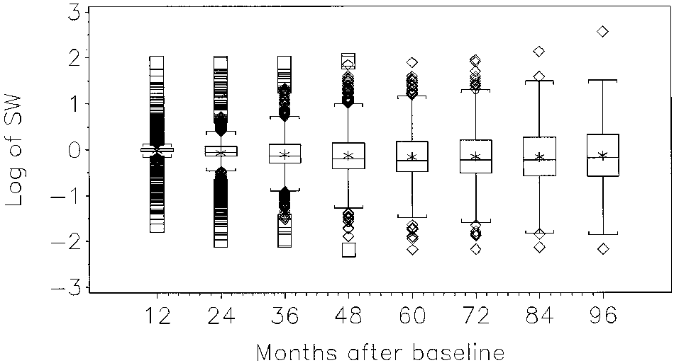
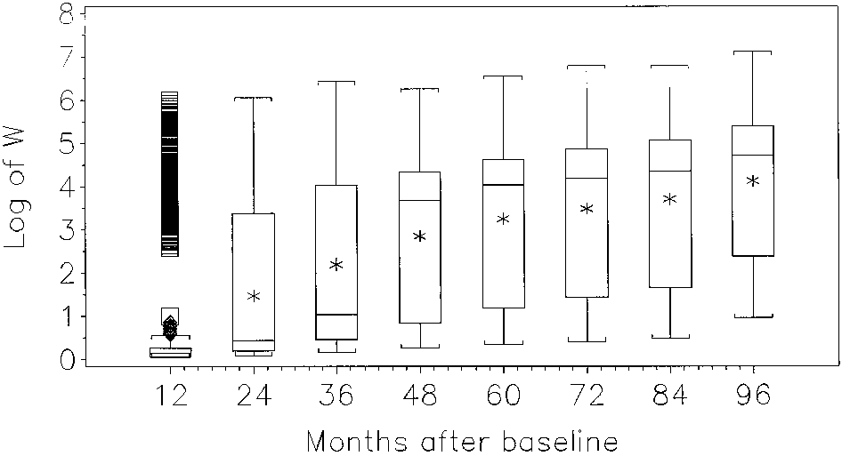
The distribution of the final weights, which combine
person having his own observed zidovudine history up to
information on zidovudine and censoring history, is pre-
month t given baseline covariates V, and, then, given
sented in Figures 1 and 2 for several follow-up times (a
also time-varying covariates L(t). Similar models were fit
logarithmic transformation was applied for display pur-
for the outcome “censoring,” after adding zidovudine
poses only). Two sets of weights were estimated: the
history as a time-varying dichotomous variable indicat-
ˆ (t) ϫ swˆ† (t) and the nonstabilized
ing whether the subject had started zidovudine by
ˆ (t) ϫ wˆ† (t). The distribution of stabilized
weights is symmetric and centered around 1 at all times,
Table 3 shows the center and dispersion parameters of
whereas its variance increases over time. The distribu-
the distribution of the four estimated probabilities at two
tion of the nonstabilized weights is skewed, and its
arbitrary time points: 24 and 84 months of follow-up.
variance greatly exceeds that of the stabilized weights. Epidemiology
ion paper,4 because the covariates in L(t) are affected byearlier treatment, the zidovudine coefficient cannot becausally interpreted as either the overall zidovudine ef-fect or the direct effect of zidovudine mediated by path-ways not through the covariates L(t). In contrast, underour assumption of no unmeasured confounders, the co-efficient of zidovudine in our marginal structural Coxmodel represents the overall effect of zidovudine.
More specifically, if we had included in the above
covariate-adjusted time-dependent Cox model both aterm for current zidovudine exposure [that is, A(t)] andseveral terms for past zidovudine exposure {for example,
FIGURE 1. Distribution of stabilized weights SW. The
cumulative months on treatment before t [cum(t)], and
box for each group shows the location of the mean (*),
the indicator A(t Ϫ 6) of whether a subject was on
median (middle horizontal bar) and quartiles (border hori-
treatment 6 months previously}, then, in the absence of
zontal bars). Vertical lines extend to the most extreme ob-
unmeasured confounders and model misspecification,
servations which are no more than 1.5 ؋ IQR beyond the
the coefficient of A(t) would have a causal interpreta-
quartiles. Observations beyond the vertical lines are plotted individually, if they lie within the limits of the frame.
tion but the coefficients cum(t) and A(t Ϫ 6) wouldnot, because only current zidovudine does not affectL(t). The coefficient of A(t) would represent the effecton a log rate ratio scale of recent zidovudine on mortalityin month t within strata defined by zidovudine andcovariate history up to t and would generally differ fromthe coefficient  of A(t) in our MSM, as the coefficients
in the two models represent different causal contrasts. [Indeed, it can be shown that if our MSM is correct and
 is nonzero, the causal rate ratio for current zidovudine
in the covariate and past treatment-adjusted time-de-pendent Cox model will not be constant over stratadefined by past treatment and covariate history. Hence,we would need to include interaction terms between
FIGURE 2. Distribution of nonstabilized weights SW. A(t) and the variables L(t), A(t Ϫ 6), and cum(t) in our
The box for each group shows the location of the mean (*),
covariate and past treatment-adjusted time-dependent
median (middle horizontal bar) and quartiles (border hori-
Cox model to avoid model misspecification.] However,
zontal bars). Vertical lines extend to the most extreme ob-
as mentioned above, the coefficient (estimated to be
servations which are no more than 1.5 ؋ IQR beyond the
0.4) of A(t) in the covariate-adjusted time-dependent
quartiles. Observations beyond the vertical lines are plotted
Cox model that does not include terms for past zidovu-
individually, if they lie within the limits of the frame.
dine exposure does not have a causal interpretation,because past treatment is a confounder for current treat-ment and thus must be adjusted for. This is true even
The weight estimates were robust with respect to the
under the null hypothesis of no direct, indirect, or over-
method used to estimate the time-dependent baseline
all effect of zidovudine on mortality whenever, as will be
logit ␣ (k) in the logistic models for zidovudine and
essentially always the case, a component of L(t), say
censoring, provided that sufficient flexibility was al-
RBC, and mortality in month t have an unmeasured
lowed. The weights in Figures 1 and 2 were obtained by
common cause (for example, the baseline number of
modeling the time-dependent intercept ␣ (k) with nat-
bone marrow stem cells); adjusting for a variable L(t)
ural cubic splines with five knots (on months 23, 44, 71,
affected by past zidovudine makes past zidovudine a
94, and 100, which correspond to the percentiles 5, 27.5,
noncausal independent (protective) risk factor for mor-
tality within strata of L(t) and A(t), and thus, to estimatethe effect of recent zidovudine exposure, past zidovudine
Adjusting for Time-Dependent Confounders in
must be controlled as a confounder in the analysis. a Cox Model We also fit a standard (unweighted) time-dependent Cox model in which we included, at each month t, the Comparison of Marginal Structural Models with
current value L(t) of the time-dependent covariates, the
Previously Proposed Methods
baseline covariates V, and the treatment A(t). We ob-
Before introducing MSMs, Robins and co-workers intro-
tained a point estimate of 0.4 (95% confidence interval-
duced three methods for estimation of the causal effect
0.3– 0.5) for the zidovudine coefficient, which was con-
of a time-varying treatment in the presence of time-
siderably less than our stabilized IPTW estimate of 0.7.
varying confounders: the parametric g-computation al-
Nevertheless, as discussed in section 7.1 of our compan-
gorithm formula estimator,12,13 g-estimation of structural
Epidemiology
nested models,12,14,15 and the iterative conditional expec-
(say k ϭ 0, 1, 2), but for large k we require strong
tations (ICE) estimator.3,12 IPTW estimation of MSMs
modeling assumptions, as there are many variables in
constitutes a fourth method. When (1) both treatment
l(k) ϭ (l(0), l(1), . . . , l(k)) and in a(k Ϫ 1). It is
and the confounders are discrete variables, (2) they are
unlikely that these modeling assumptions would be pre-
measured at only a few time points, and (3) the study size
cisely correct. Furthermore, even when these modeling
is large, then estimation can be carried out using fully
assumptions are correct, if the distribution of the stabi-
saturated models (that is, nonparametrically), and all
lized weights is highly variable and skewed as a result of
four methods are precisely equivalent. They differ when,
very strong covariate-treatment associations, 95% con-
owing to sparse multivariate data, one must introduce
fidence intervals based on IPTW estimation of an MSM
will be very wide and may fail to cover the true param-
ICE estimators can only rarely be used, because they
eter at least 95% of the time, unless the sample size is
often lead to logically incompatible models and will not
be discussed further.12 Of the remaining three methods,
The use of g-estimation of SNMs overcomes the
inference based on SNMs and MSMs is preferable to
above difficulties. For example, one can use SNMs to
that based on the parametric g-computation algorithm.
estimate the effect of an exposure on mortality in occu-
The reason is that MSM and SNM models, in contrast
pational cohort studies.14,16 Similarly, one can unbi-
to models based directly on the conditional probabilities
asedly estimate the causal parameter of a SNM without
in the g-computation algorithm formula, include param-
having to model the probability of treatment given the
eters that represent the null hypothesis of no treatment
past through end of follow-up. Instead, in the setting of
effect.12,15 As a consequence, when using the parametric
a discrete A(k) and L(k) described above, one can un-
g-computation algorithm estimator, it is quite difficult to
biasedly estimate the parameters of SNMs by using a
determine whether one’s confidence interval for the
saturated model for the probability of exposure A(k)
treatment effect includes the null hypothesis of no ef-
given the past for k ϭ 0,1,2 periods and ignoring expo-
sure at later periods, thus preventing bias due to mis-
MSMs have two major advantages over SNMs. Al-
specification of the model for exposure. Of course, as
though useful for survival time outcomes, continuous
always in statistical analysis, there will be a loss of
measured outcomes (for example, blood pressure), and
efficiency of estimation associated with this protection
Poisson count outcomes, logistic SNMs cannot be con-
against bias. Finally, in the presence of strong covariate-
veniently used to estimate the effect of treatment on
treatment associations, theoretical arguments imply that
dichotomous (0, 1) outcomes unless the outcome is
it should be possible to construct confidence intervals
rare.1,2,12 This is because logistic SNMs cannot be fit by
based on g-estimation of SNMs that are both narrower
g-estimation. In contrast, as we have seen,4 IPTW esti-
and have better coverage properties than those based on
mation of logistic MSMs can be used to estimate the
IPTW estimation of MSMs. However, further research is
effect of a time-dependent treatment on a binary out-
required to see whether this theoretical prediction is
The second major advantage of MSMs is that they
Another advantage of SNMs over MSMs is that,
resemble standard models, whereas SNMs do not. For
although MSMs are useful for estimating the causal
example, the logistic MSM described in our companion
effect of the prespecified treatment regime a (for exam-
paper4 and the Cox proportional hazards MSM described
ple, always treat, treat on alternate months, etc), they
here are the natural way to extend the ordinary logistic
are much less useful than SNMs for modeling the inter-
and time-dependent Cox models to allow for estimation
action of treatment with a time-varying covariate and
of causal effects. The close resemblance of MSMs to
for estimating the effect of dynamic treatment plans in
standard statistical models makes their application more
which treatment on a given month is decided in part on
intuitive for researchers and easier for programmers.
the basis of a subject’s evolving covariate history.1,2 It is
Nevertheless, SNMs have a number of advantages
important to recognize that actual medical treatment
over MSMs. For example, as discussed in Ref 4, MSMs
regimes are usually dynamic, because if a patient devel-
should not be used to estimate effects in studies (such as
ops a toxic reaction to a drug, the drug must be stopped.
occupational cohort or cancer screening studies) in
Nonetheless, causal questions concerning prespecified
which, at each time k there is a covariate level l(k) such
treatment plans, such as estimating the effect of a con-
that all subjects with that level of the covariate are
tinuous exposure at a certain level vs no exposure, are of
certain to receive the identical exposure a(k).1,2
great interest in many areas of epidemiology, including
A second major drawback of MSMs is that one must
be able to specify a correct model for the conditionalprobability of exposure,
Discussion pr͑ A͑k͒ ϭ a͑k͉͒L͑k͒ ϭ l͑k͒, A͑k Ϫ 1͒ ϭ a͑k Ϫ 1͒͒,
We have used a marginal structural Cox proportionalhazards model to estimate the causal effect of zidovudine
for each time k up to end of follow-up. This is unfortu-
on mortality of HIV-positive patients in the MACS.
nate because, if the L(k) and A(k) are discrete, we could
This method was used because standard statistical meth-
use nonparametric saturated models for small values of k,
ods are not appropriate when there exists time-depen-
Epidemiology
dent confounding by variables, such as CD4 count, that
are less restrictive than those of standard methods;
MSMs do not require the absence of time-dependent
Because of the presence of confounding, the crude
confounding by variables affected by previous exposure.
mortality rate ratio for zidovudine was 3.6 (95% confi-dence interval-3.0 – 4.3), erroneously suggesting thatzidovudine increased risk of death. The rate ratio esti-mated by the (unweighted) standard model that in-
Acknowledgments
cluded only baseline covariates, and that therefore does
We thank Sander Greenland and several referees for helpful comments.
not adjust for time-dependent confounding, was 2.3
Data in this manuscript were collected by the Multicenter AIDS Cohort
(95% confidence interval-1.9 –2.8), which still suggests
Study (MACS) with centers (Principal Investigators) at The John HopkinsSchool of Public Health (Joseph Margolick, Alvaro Mun˜oz); Howard Brown
Health Center and Northwestern University Medical School (John Phair);
In fact, the mortality rate ratio for zidovudine was 0.7
University of California, Los Angeles (Roger Detels, Janis V. Giorgi, Beth
(95% conservative confidence interval-0.6 –1.0) in the
Jamieson); and University of Pittsburgh (Charles Rinaldo). The MACS isfunded by the National Institue of Allergy and Infectious Diseases, with addi-
weighted analysis that provides, under our assumptions,
tional supplemental funding from the National Cancer Institute: UO1-AI-
an unbiased estimate of the causal rate ratio, exp( ), of
35042, 5-M01-RR-00052 (GCRC), UO1-AI-35043, UO1-AI-37984, UO1-AI-
the marginal structural Cox model, because the
35039, UO1-AI-35040, UO1-AI-37613, UO1-AI-35041.
weighted analysis appropriately adjusts for time-depen-dent confounders affected by earlier treatment.
The difference between the unweighted and weighted
estimates is an indication of the amount of confounding
References
due to the time-dependent prognostic factors. The
1. Robins JM. Marginal Structural Models. 1997 Proceedings of the Section on
weights can be interpreted as the number of copies of
Bayesian Statistical Science. Alexandria, Virginia: American Statistical
each observation that are necessary to form a pseudopo-
2. Robins JM. Marginal structural models versus structural nested models as
pulation in which censoring does not exist and in which
tools for causal inference. In: Halloran E, Berry D, eds. Statistical Models in
the time-dependent prognostic factors do not predict
Epidemiology: The Environment and Clinical Trials. New York: Springer-
initiation of zidovudine history (that is, treatment is
3. Robins JM. Structural nested failure time models. In: Andersen PK, Keiding
N, section eds. Survival Analysis. In: Armitage P, Colton C, eds. The
Like all causal inferences, the validity of our analyses
Encyclopedia of Biostatistics. Chichester, UK: John Wiley and Sons, 1998;
depends on a number of assumptions. First, we assume
that the information on month of zidovudine initiation
4. Robins JM, Herna´n MA, Brumback B. Marginal structural models and causal
inference in epidemiology. Epidemiology 2000;11:550 –560.
and month of death is accurate. Second, we assume that
5. Kaslow RA, Ostrow DG, Detels R, Phair JP, Polk BF, Rinaldo CR. The
the measured covariates in L(t) are sufficient to adjust
Multicenter AIDS Cohort Study: rationale, organization, and selected char-
for both confounding and selection bias due to loss to
acteristics of the participants. Am J Epidemiol 1987;126:310 –318.
6. Graham NM, Zeger SL, Park LP, Vermund SH, Detels R, Rinaldo CR, Phair
follow-up. This assumption implies that we have avail-
JP. The effects on survival of early treatment of human immunodeficiency
able, for each month t, accurate data recorded in L(t) on
virus infection. N Engl J Med 1992;326:1037–1042.
all time-dependent covariates that (1) are independent
7. Robins JM. Causal inference from complex longitudinal data. In: Berkane
M, ed. Latent Variable Modeling and Applications to Causality: Lecture
predictors of death and (2) independently predict the
Notes in Statistics 120. New York: Springer-Verlag, 1997;69 –117.
probability of starting zidovudine and/or of being cen-
8. Kinloch-De Loes S, Hirschel BJ, Hoen B, Cooper DA, Tindall B, Carr A,
sored in that month. Unfortunately, as in all observa-
Saurnt JH, Clumeck N, Lazzarin A, Mathiesen L, et al. A controlled trial ofzidovudine in primary human immunodeficiency virus infection. N Engl
tional studies, these two assumptions cannot be tested
from the data. In our analysis, we assume that this goal
9. D’Agostino RB, Lee M-L, Belanger AJ. Relation of pooled logistic regression
has been realized, while recognizing that, in practice,
to time dependent Cox regression analysis: the Framingham Heart Study. Stat Med 1990;9:1501–1515.
this assumption would never be precisely or sometimes
10. Liang K-Y, Zeger SL. Longitudinal data analysis using generalized linear
even approximately true. Recently, Robins et al.16 have
developed extensions of IPTW estimation of MSMs that
11. Hastie TJ, Tibshirani RJ. Generalized Additive Models. New York: Chap-
allow one to evaluate the sensitivity of one’s estimates to
12. Robins JM. Correction for non-compliance in equivalence trials. Stat Med
increasing violation of these fundamental assumptions.
Third, we assume that the models for initiation of
13. Robins JM. A graphical approach to the identification and estimation of
zidovudine and censoring, given the past, are correctly
causal parameters in mortality studies with sustained exposure periods. J Chron Dis 1987;40(suppl. 2):139S–161S.
specified. Fourth, we assume that our MSM for the effect
14. Robins JM, Blevins D, Ritter G, Wulfsohn M. G-estimation of the effect of
of zidovudine on mortality, within levels of baseline
prophylaxis therapy for Pneumocystis carinii pneumonia on the survival of
covariates V, is correctly specified.
AIDS patients (erratum in Epidemiology 1993:4;189). Epidemiology 1992;3:319 –336.
Although the stated assumptions may seem heroic,
15. Robins JM. The analysis of randomized and non-randomized AIDS treat-
note that in point-exposure studies the same assump-
ment trials using a new approach to causal inference in longitudinal studies.
tions (accurate information, no unmeasured confound-
In: Sechrest L, Freeman H, Mulley A, eds. Health Service Research Meth-odology: A Focus on AIDS. Rockville, MD: National Center for Health
ers, noninformative censoring, and no misspecification
Services Research, U.S. Public Health Service, 1989;113–159.
of the model) are required to give a causal interpretation
16. Robins JM, Rotnitzky A, Scharfstein DO. Sensitivity analysis for selection
to the parameters of standard statistical models. Further-
bias and unmeasured confounding in missing data and causal inferencemodels. In: Halloran E, Berry D, eds. Statistical Methods in Epidemiology:
more, when studying the effect of a time-dependent
The Environment and Clinical Trials. New York: Springer Verlag, 1999;1–
treatment such as zidovudine, the assumptions of MSMs
Epidemiology APPENDIX
model 4 includes the time-dependent covariates (to
For each model, we output a new data file (option
In this appendix, we provide SAS code to fit the Cox
“out ϭ” in Proc Logistic) that contains, for each person-
proportional hazards MSM described in the text. The
month, the original variables plus the predicted values
original MACS data file contains one record per man,
from the model (option “pϭ”). As an example, the first
but here we use a transformed, or pooled, file (MAIN)
Proc Logistic creates the data set MODEL1 with itspredicted values as the variable PZDV0.
with each person-month as a separate record. This file
In the following data step, we merge the four output
format is necessary to fit pooled logistic models. The
files in the file MAINW that contains the predicted
code used to generate the pooled dataset from the orig-
values from the four logistic models. We then compute
inal one is available from the first author upon request.
the numerator K20 and the denominator K2W of the
The records in the file MAIN must be sorted by patient
sw† (t) from models 3 and 4.
identification number (variable ID) and, within each ID
iSimilarly, we calculate the numerator K10 and the
level, by month of follow-up (MONTH).
denominator K1W of the weights sw (t) for months in
The SAS code shown below is organized as follows.
which the subject has not yet started zidovudine from
First, we use Proc Logistic to fit four pooled logistic
models 1 and 2. For a month in which a subject did
models (two for the probability of remaining off zidovu-
begin zidovudine, we multiply by 1 minus the predicted
dine and two for the probability of remaining uncen-
value. For months subsequent to starting zidovudine, we
sored) and obtain their predicted values. Second, we use
no longer update K10 and K1W. Then we use the
a SAS data step to calculate the weights for each person-
numerators and denominators to calculate the “stabi-
month from the predicted values of the previous four
lized” weights sw (t) ϫ sw† (t) (STABW), and use the
models. Last, we use Proc Genmod to fit the final
denominators alone to calculate the “nonstabilized”
weighted pooled logistic model that estimates the causal
weights w (t) ϫ w† (t) (NSTABW).
parameter of interest and its robust standard error.
Finally, we call Proc Genmod to fit a weighted pooled
The outcome variable in models 1 and 2 is a dichot-
logistic model for survival to obtain consistent estimates
omous variable A indicating whether the patient had
of the parameters of our Cox MSM. The outcome vari-
started (A ϭ 1) or remained off (A ϭ 0) zidovudine on
able of this model, D, is a dichotomous variable indicat-
that month. When the option “descending” is not spec-
ing whether the patient died (D ϭ 1) or remained alive
ified, Proc Logistic models the probability that the out-
(D ϭ 0) in that month. The program will provide robust
come variable is 0. Hence, models 1 and 2 model the
standard errors for the model parameters when the op-
probability of remaining off zidovudine. The “where”
tion “repeated” is included. The patient identification
statement restricts the analysis to patients not previously
variable and the independent working correlation ma-
on zidovudine by specifying that either month of fol-
trix (“subject ϭ ID/type ϭ ind”) must be specified. We
low-up (MONTH) is less than or equal to month of
fit the model using the stabilized weights by specifying
onset of zidovudine (ZDVM) or zidovudine was never
the variable STABW in the “scwgt” statement. Speci-
initiated during the follow-up period (ZDVM is coded
fying the variable NSTABW fits the model with non-
as missing, if this is the case). Model 1 includes as
regressors a time-dependent intercept and the baseline
The SAS code given below can also be used to fit the
covariates V: baseline age, calendar year, CD4, CD8,
logistic MSM of our companion paper.4 The only differ-
WBC, RBC, platelets, and presence of symptoms. Model
ence is that the final weighted logistic model in Proc
2 includes, in addition, the time-dependent covariates
Genmod includes a single observation per person using
L(t): most recently available CD4, CD8, WBC, RBC,
as outcome variable the logistic variable Y of our com-
platelets, symptoms, and AIDS-defining illness. We es-
panion paper, rather than the survival variable D con-
timate the time-dependent intercept by a smooth func-
tion of the time since beginning of follow-up (MONTH)using natural cubic splines with five knots. To do so, we
need to include, as regressors, the variables MONTH1,
MONTH2, and MONTH3, that are specific polynomial
functions of MONTH (calculated with the cubic splines
model AϭAGE0 YEAR01 YEAR02 YEAR03
SAS macro RCSPLINE in survrisk.pak, by Frank Harrel,
which is publicly available on http://jse.stat.ncsu.edu:70/
The outcome variable in models 3 and 4 is a dichot-
omous variable C indicating whether the patient was
censored (C ϭ 1) or uncensored (C ϭ 0) in that month.
Thus, models 3 and 4 model the probability of remaininguncensored for each person-month. All available per-
son-months are used. Model 3 includes the baseline
covariates and the time-dependent intercept, whereas
Epidemiology
model AϭAGE0 YEAR01 YEAR02 YEAR03
/* reset the variables for a new patient */
k10ϭ1; k20ϭ1; k1wϭ1; k2wϭ1;
/* Inverse probability of censoring weights */
/* Inverse probability of treatment weights */
/* patients not on zidovudine */if zdvmϾday or zdvm ϭ. then do;
model CϭA AGE0 YEAR01 YEAR02 YEAR03
/* patients that start zidovudine this month */
/* patients that have already started zidovudine */
model CϭA AGE0 YEAR01 YEAR02 YEAR03
/* Stabilized and non stabilized weights */
CD41 CD42 CD81 CD82WBC1 WBC2 RBC1 RBC2
PLAT1 PLAT2 SYMPT AIDSMONTH MONTH1-MONTH3;
model DϭA AGE0 YEAR01 YEAR02 YEAR03
/* variables ending with 0 refer to the numerator of the
variables ending with w refer to the denominator of
Artikel erschienen bei Leben wie zuvor, Schweizer Verein für Frauen nach Brustkrebs, Bulletin 65, Sonderausgabe Aromatasehemmer in der modernen Brustkrebstherapie Erstes Behandlungsziel bei Brustkrebs im Frühstadium ist immer die vollständige operative Tumorentfernung. Moderne Operationstechniken und systemische Behandlungen machen heutzutage in zwei von drei Fällen Brust erhalten
CEE Bulletin on Sexual and Reproductive Rights No 8 (30) 2005 table of contents: http://www.astra.org.pl/30_issue.htm (1 van 7)16-1-2006 12:17:07 BURNING ISSUE - 2005 World Summit In this Burning Issues will provide you with diversity of information related to upcoming September Millennium Summit + 5 which is expected to be the largest gathering of world leaders in history. 2005
 Epidemiology